Equilibrium Occupancy:

Consider an ecosystem which is composed of a bunch of individual cells or areas. Within each cell or areas one can identify 3 possible conditions

• the cell is occupied by females; we will call this condition p .

• the cell is habitable but is currently not occupied; we will call this condition h .

• The cell is unfit for habitation X

The basic assumptions in the following methodology are:

• All females succesfully mate
• Females die in random locations in the ecosystem
• Juveniles disperse prior to reproduction and their survival is density dependent based on the probability of finding a suitable habitat in a relatively large territory before dying from starvation or predation

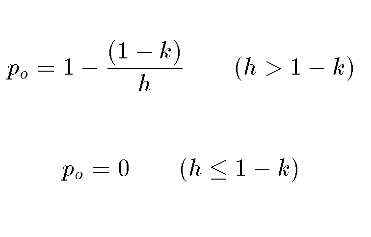
In general, a species will not inhabit all of the available habitat as that could lead to extinction (as in the classic overgrazing scenario). A working model is that habitable and uninhabitable patches of land are randomly dispersed throughout the ecosystem. This model makes an important prediction for p_o which is the equilibrium occupancy of suitable habitat by females (the model assumes the males will find them ...) and it has two parameters

• h is the proportion of the region which is habitable
• k is the demographic potential of the species.

Demographic potential gives the maximum proportion of habitat occupied at equilibrium in a completely suitable region.

Even in a completely suitable region, not all habitat is occupied because some time elapses before a territory vacated by the death of the resident female is reclaimed by a random walking juvenile.

Furthermore, as the amount of suitable habitat decreases, the equilibrium occupancy declines to eventually reach an "extinction threshold". This represents the minumum proportion of suitable habitat necessary to sustain the population.

For species with high demographic potential (high numeric values of k), the equilibrium occupancy rapidly declines as the amount of suitable habitat decreases.

k is not something easily measured but p and h can be. These are related by the following:

Doing a little algebra reveals that

k = (ph) -h + 1

The difference between p and p_o is not important; p_o refers to the statistical equilibrium population that is time averaged; p refers to a snapshot in time (e.g. when the system was sampled). In general, in the real world, ecosystems are never sampled well enough in time for p_o to be properly determined and hence we just use p .

Note that in the unique case of h = 1 (i.e. 100% of the ecosystem is habitable), then p (the observed occupancy) will equal k and the species is at is demographic potential.

More generally, lets consider a case of h = 0.5 for a species with k = 0.7. In that case, we should observe a value of

p = 1 - 0.3/0.5 = 0.4

So 40% of this ecosystem should be occupied by adult females if it is in equilibrium.

If h is known exactly (which we will pretend that it is) then the variance in k can be determined as follows:

where N_p is the number of suitable territories (grids) that have been observationally sampled for occupancy and/or suitability.

Example:

Below is a dataset with N_p = 20. That is 20 habitat cells have been sampled within the entire ecosystem. From that sample we find:

• p = 0.3 (that is 6 cells had females in them)
• h = .45 (9 out of 20 cells are habitable)
• x=5 (5 cells are not habitable)

From this, we now solve for k.

Putting in the values for p and h and solving for k shows that k =0.685 meaning that 68.5% of the total ecosystem is, in principle, habitable.

The standard deviation of k (which is the square root of the variance) would be:

• σ_p² =0.3(1-0.3)/20 = 0.011
• σ_k² = (0.45)²*(0.011) = 0.0022
• σ_k = .047

And therefore k is determined to an accuracy of 4.7% k = 0.685 +/- 0.047.

With our sample determination of k, we can now extrapolate to the whole ecosystem, which is the point of this statistical approach.

If we assume, for the sake of argument, that before development, h was 0.65 then that would lead to p = 1 - .315/.65 = 0.525 compared to the current value of p = 0.3.

On this basis, one could therefore argue that development has lead to a substantial reduction of the species throughout the ecosystem as the observed value of p is much less than the theoretical value of p prior to habitat augmentation.

However, this is now where you have to consider the error bars on k and this is the crucial intersection between science and policy. This is not part of the how the spotted owl decisions have been made, but is potentially a big effect.

To wit,

Suppose that k really is .755 (1.5 standard deviations above our estimate and therefore about 10% likely)

Then the theoretical value of p is (1 - .245/.65 = .375) which is closer to our observed value of 0.3 and thus our statement above in red has less significance.

This point is absolute crucial. Knowledge of k is fundamental and errors in k are extremely important. Do not forget this. Ever.

Therefore, in the real world, its important to be able to determine k to pretty high accuracy.

Finally we consider the critical case of h = 1 - k . (refer to the equation for p above, if h = 1-k then p = 1-1 = 0.

If h in the real world falls below this critical value, then the species will no longer have enough habitat to support them.

Formally, for k = 0.685 we would get h_critical = 1 - 0.685 = 0.315 which is less than the present h of 0.45.

That means you could argue that 13.5% (.45 - .315) more of the total ecosystem could be developed without killing the species.

However, once again, errors on k are important. If you use a k = .615 (again allowed by the data) this gets you to h_critical = 0.385 meaning only 6.5% of the remaining habitat can be lost

So unless you know k very accurately, you can not determine with accuracy the real world value of h_critical

This means you can easily make mistakes and develop too much habitat. This happens time and time again. Why? Because the errors in the measurments are not properly factored in at the time of policy decision.

Only the average value is used.

A species that does not understand its errors and how to apply that to public policy deserves its fate.