The KS Statisical Test

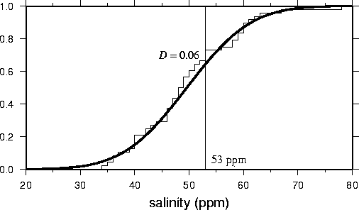
This is a powerful test that lets you compare two distributions or to compare a distribution to a model. It is more powerful than the chi² since it doesn't involve binning the data or calculating expected frequencies at discrete points.

The fundamental tool in the KS test involves constructing a cumulative frequency distribution from the data and or model.

Most importantly, the KS test allows one to compare arbitrary distributions to one another. That is, the distributions do not have to be normal. This is quite important.

For instance, a standard statistical test, called the t-test assumes a normal distribution, and the only thing that changes is the sample mean. If the sample sizes are large, then the t-test is robust (CLT). But if its small (usually N < 40) it can produce misleading results (e.g. this is how to make statistics lie).

So let's start off with an example with low N and make use of the Histogram Applet

Sample A: (mean = -0.16) ; (stdev = 1.11); (error in mean = 0.25)

0.22
-.87
-2.39
-1.79
.37
-1.54
1.28
-.31
-.74
1.72
.38
-.17
-.62
-1.10
.3
.15
2.3
.19
-.5
-.09

Sample B: (mean = 0.97); (stdev = 3.97); (error in mean = 0.89)

-5.13
-2.19
-2.43
-3.83
.5
-3.25
4.32
1.63
5.18
-.43
7.11
4.87
-3.10
-5.81
3.76
6.31
2.58
0.07
5.76
3.50

The t-test (or in the one sided case this is called the Z-test) compares the differences in the means. This test assumes that the underlying distributions are normal for each sanmple. In this case, they are clearly not, so we can't use this test. Well, let's just pretend that we can: (note, that the standard deivation of a sample of numbers has no meaning if the distribution is far from normal - this is why this doesn't work)

For Sample A: the Mean is -0.16 and the uncertainty in the mean is the standard deviation divided by the square root of N (in this case N = 20)

So sample A is -0.16 (M1) +/- 0.25 (E1)

Sample B is 0.97 (M2) +/- 0.89 (E2)

The statistic is:

Doing the math leads to a result of 1.24 for the statisic. Normally the value would have to exceed 3 to use this test to show the distribution are not the same. So the t-test fails in this case, but our other test, coming below, would not fail.

Let's look at this sample.

Sample C:

1.26
.34
.7
1.75
50.57
1.55
.08
.42
.50
3.20
.15
.49
.95
.24
1.37
.17
6.98
.10
.94
.38

Now clearly this data set has an outlier that totally biases the descriptive statistics (mean =3.6; sd = 10.9). In a normal distribution one expects 15% of the data to lie below 1 standard deviation so in this case that would be below 3.60-10.9 = -7.5 but in fact there are no data values below 0 so something funny is going on.

So let's construct a cumulative fraction function. Sorting the data from min to max helps with this:

.08
.10
.15
.17
.24
.34
.38
.42
.49
.50
.70
.94
.95
1.26
1.37
1.55
1.75
3.20
6.98
50.57

Remember N = 20 so in this case there are 13 (65%) points below a value of 1. Similarly 85% of the data have values below 2. So the cumulative fraction plot will look like this:

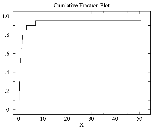
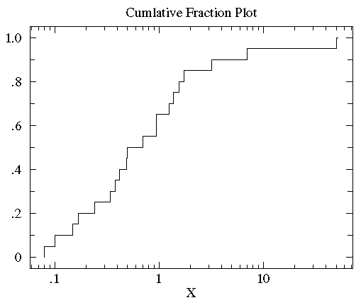
If you change the X-axis to be logarithmic the form of the distribution becomes more well defined and its easier to see where the median is (.5).

Okay, fine, so what's the test?

Now we have another sample, sample D, which is related to sample C.

0.11
0.18
0.23
0.51
1.19
1.30
1.32
1.73
2.06
2.16
2.37
2.91
4.50
4.51
4.66
14.68
14.82
27.44
39.41
41.04

Are the distribution of data values different between D and C?

Plot both cumulative frequency distributions on the same graph and find the maximum difference as shown below:

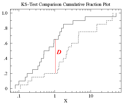
What is denoted as D is the KS statistic. In this case D=.45 and occurs at a value of log X =1. The formal probability result (see calculator link below) is that these two distributions are different at the P=.023 (i.e. 97.7% confidence level)

And finally, here is an example from real life.

Two near-by apple trees are in bloom in an otherwise empty field. One is a Whitney Crab the other is a Redwell. Do bees prefer one tree to the other? We collect data by using a stop watch to time how long a bee stays near a particular tree. We begin to time when the bee touches the tree; we stop timing when the bee is more than a meter from the tree. (As a result all our times are at least 1 second long: it takes a touch-and-go bee that long to get one meter from the tree.) We wanted to time exactly the same number of bees for each tree, but it started to rain. Unequal dataset size is not a problem for the KS-test.

whitney={16.5, 1, 22.6, 25.3, 23.7, 1, 23.3, 23.9, 16.2, 23.0, 21.6, 10.8, 12.2, 23.6, 10.1, 24.4, 16.4, 11.7, 17.7, 34.3, 24.3, 18.7, 27.5, 25.8, 22.5, 14.2, 21.7, 1, 31.2, 13.8, 29.7, 23.1, 26.1, 25.1, 23.4, 21.7, 24.4, 13.2, 22.1, 26.7, 22.7, 1, 18.2, 28.7, 29.1, 27.4, 22.3, 13.2, 22.5, 25.0, 1, 6.6, 23.7, 23.5, 17.3, 24.6, 27.8, 29.7, 25.3, 19.9, 18.2, 26.2, 20.4, 23.3, 26.7, 26.0, 1, 25.1, 33.1, 35.0, 25.3, 23.6, 23.2, 20.2, 24.7, 22.6, 39.1, 26.5, 22.7}

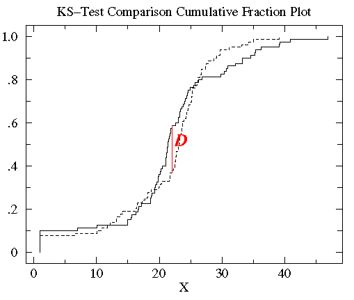
In this case, standard statistical tests would fail to find a difference between this two distributions but the KS test can.

Enter the data (cut and paste) into the highly useful KS Test Calculator.

The statistic for this example is D = 0.2204.

Specifically the result is a 96.5% chance of these distributions being different. That is the bees prefer one tree over another.

General formula for computing the KS statistic:

"One Sided" (comparing a data distribution to a model one, like a normal distribution) - in fact the KS test is the BEST test to determine if you sample actually is consistent with a normal distribution. The KS test can not be used on data samples with less than about 10 values since you can't really construct a realiably cumulative freq. distribution.

For N > 10:

• .05 level = 1.36/sqrt N
• .01 level = 1.63/sqrt N

"Two Sided" (comparing two different data distributions or size m and n)

• .05 level = 1.36(sqrt((m+n)/mn)
• .01 level = 1.63(sqrt((m+n)/mn)

  For the case of m=n=80 the values are 0.215 and 0.257.

  So, at the 95% confidence level I can say the two distributions are *not* the same since .221 > .215; however, I can not say this at the 99% confidence level.

  The other very useful feature of the KS test (which will explore in excel) is testing the data against a model. An example is shown here: