 a good example of non-linear
feedbacks in ecosystems.
a good example of non-linear
feedbacks in ecosystems.
Biologists like to talk a lot about r-selected (growth selected) and k-selected (carrying capacity limited) species usually in the context of predator-prey relations.
a good example of non-linear
feedbacks in ecosystems.
Biologists like to talk a lot about r-selected (growth selected) and k-selected (carrying capacity limited) species usually in the context of predator-prey relations.
More specifically:
K-selected species usually live near the carrying capacity of their environment. Their numbers are controlled by the availability of resources. In other words, they are a density dependent species. Food availability is one resource that controls population size, especially if the food is relatively localized.
The attributes of a K-selected species include a long maturation time, breeding relatively late in life, a long lifespan, producing relatively few offspring, low mortality rates of young, and extensive parental care. Examples of a K-selected species include elephants, apes and humans.
The attributes of a r-selected species include a short maturation time, breeding at a young age, a short lifespan, producing many offspring quickly, small offspring, high mortality rates of young, and nonexistent parental care. Examples of r-selected species include waterfleas, insects, and rabbits.
r and K selection may depend on ecosystem condition:
While r vs K selection is a useful framework it generally oversimplifies the
problem. Most real systems are subject to non-linear or chaotic
dynamics, involving unstable oscillations around points of
equilibrium.
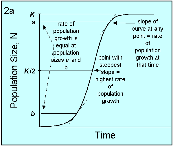
K-selected species are idealized by the equation below where it
can be seen that the growth rate, R, becomes zero as N approaches
K. This is called negative feedback - the idea being as
conditions get "crowded" it is detrimental to growth. The problem
with real systems is that estimates of K are very difficult and
uncertain:
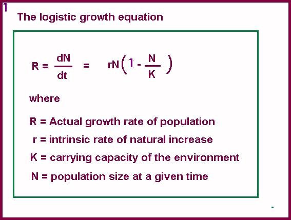
Note when N << K, N/K is zero. In this case pure (unbounded) exponential growth is occuring:
(Note: Despite what you may have heard in other ENVS classes, human growth is occuring in a mathematically exponential way, on a logistic growth curve - this represents bounded exponential growth)
r-growth is standard exponential growth which leads to population crashes. The functional difference between r and K selected growth is shown below:
In reality, K-selected growth qualitatively looks like this:
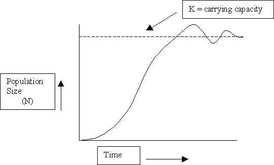
In this case we have r-selected growth up to the carrying capacity line but then we have oscillations about that line. These oscillations have points of unstable equilibria (i.e. the smaller scales peaks and valleys). Small perturbations in the system, when species growth is at one of these points, could trigger catastrophic continued r-growth or rapid decay. This is called non-linear dynamics (sometimes called chaotic dynamics).
Let's try an example with US population growth
In non-linear dynamics, small perturbations in some system can cause large changes in overall system evolution.
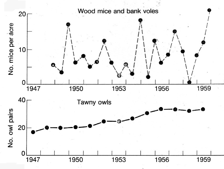
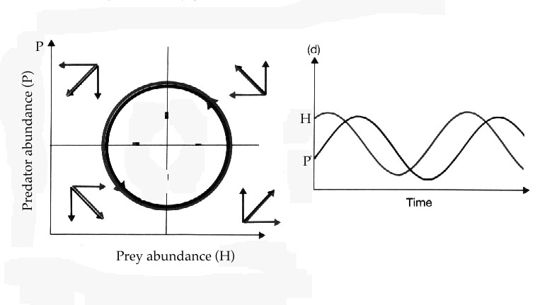
Some of this behavior is seen in the classic predator-prey case study of Lynxs and Snowshow hares. Its an excellent example of density dependent lag time in some system:
Note that this system is in quasi-equilibrium when averaged over long timescales. This is called Statistical Equilibrium .
On short time scales, however, the relative species densities are rapidly changing. Each peak or valley in this cyclical behavior is a point of unstable equilibrium and a small pertubation could drive the system completely out of control.
An additional complication is time lags or system response. In real life, this is the limiting factor for accurate modeling.
Non-linear dynamics is very difficult to accurately model because of the degree of non-linear response of the system is unknown and the relevant stress parameters are poorly understood.
But it can be effectively simulated.
density dependent lags and
note that total shark population is down
But things are that simple as outside influences can change the vectors. Dependent on what quadrant that influence operates in, the situation can be quite dramatic.
How to do simple modeling:
The simple model is that predator-prey interactios affect predator density and prey densities and then there is feedback between the two populations based on their densities.
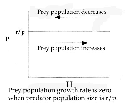
Prey Population growth rate:
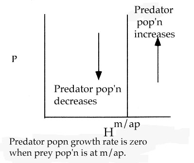
Predator population growth rate:
N = Noert
so this is how predator and prey density
enter into this.
like p, this is an efficiency
(called a conversion efficiency or a below) and is a number between 0 an 1.
This predation model is called the Lotka Volterra model (in case you want to Google on it).
The model has two equations, one for prey populations and one for predator populations. To understand dynamics, find points when populations are in equilibrium (population growth rates of zero).
Thus r/p is a controlling parameter
For predators, dP/dt=0 when apHP=mp or H=m/ap
Thus m/ap is a controlling parameter
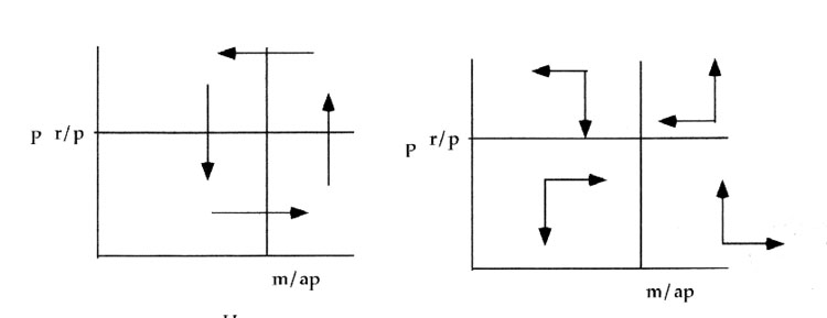
Starting from lower left quandrant and moving counter clockwise.
P falls and H grows
Additional Resources for you to Read on the LV model:
Note, what we call parameters a,m and p maybe denoted by other symbols in these other descriptions.