Buzzard Nests

Testing some empirical data against a Poisson distribution

It is often interesting to know if some event has a pattern in time or space. The pattern may be regular (evenly spaced) or aggregated ('clumps' of events). The existence of a pattern suggests that there is probably an interesting biological process at work. If there is no pattern the events will conform to a random distribution. Therefore, the first stage in the identification of a pattern is to determine if it is random. If the pattern is random it will conform to a Poisson distribution.

For example, we may be interested in the spatial arrangement of buzzard Buteo buteo nests.

In order to determine if the observed data match those expected from the theoretical (Poisson) distribution a goodness of fit test is used. In other words, we are going to use Poisson statistics to generate our expected frequencies

Begin by setting up two hypotheses, for example:

Ho : Buzzard nests are randomly distributed
H₁ : Buzzard nests are not randomly distributed

The Ho could be tested by collecting data from a number of squares of equal area. In each square the number of nests is counted. (The results are tabulated in a frequency table). In this example 60 squares were assessed. So, for example 1 nest in a square was observed 22 times; 2 nests in a square were observed 15 imtes; 4 squares had no nests, etc, etc.

X(No.of Nests)	Observed Frequency	No.of Nests
0	4	0
1	22	22
2	15	30
3	10	30
4	7	28
5	2	10
Sum =	60	120

 

Average number of nests per square = 120 / 60 = 2.00 (the sample mean )

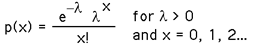
This figure, the mean of the sample (), is our best estimate of µ the true mean. Substituting this value into the Poisson equation enables the probability of observing 0, 1, 2 etc. nests per square to be calculated. The steps are summarised below.

1. Assume that nests are randomly distributed with a mean of 2.00 nests per square.

2. Use the Poisson equation to find P(0), P(1), P(2) etc., nests per square.

3. Convert these probabilities to expected numbers of squares by multiplying the probabilities by the number of surveyed squares. For example, if P(1) = 0.25 (25% chance of finding 1 nest per square) the expectation is that 25% of the surveyed squares would contain one nest as long as the number of nests per square was random with a mean of 2.00 nests per square.

   In this case 60 x 0.25 = 15.

Example for X=3:

• e^-2 = .1353
• 2³ = 8
• 3! = 6
• (.135*8)/6= .1804

Results

X(No. of Nests)	P(X)	P(X)x60
0	0.1353	8.12
1	0.2707	16.24
2	0.2707	16.24
3	0.1804	10.83
4	0.0902	5.41
5	0.0526	3.16

 

Note that the sum of P(x) = 1 because only discrete events from 0 to 5 are allowed in this data. Apparently its physically impossible to have 6 nests per square meter due to nest size or perhaps buzzard social dynamics.

In order to determine if the nests are randomly distributed it is necessary to determine if the differences between what was observed and what is expected, given a random distribution, are significant.

• If these differences are significant there is evidence that the pattern of buzzard nests is not random.
• It is also possible that the pattern could be random and any differences between observed and expected frequencies have arisen by chance.

Well we know how to test for this:

The intermediate calculations needed for this test are shown below

X	observed	expected	obs-exp(O-E)	(O-E)2/E
0	4	8.12	-4.12	2.09
1	22	16.24	5.76	2.04
2	15	16.24	-1.24	0.09
3	10	10.83	-0.83	0.06
4	7	5.41	1.59	0.46
5	2	3.16	-1.16	0.42

 

Using the data above = 2.09 + 2.04 + 0.09 + 0.06 + 0.46 + 0.42 = 5.181.

Note that most of chi² sum comes from the first two events (0 and 1) and there could be counting/measuring error involved there so one might expect the largest fluctuations to occur there.

How many degrees of freedom?

Well since there can't be 6 nests, then we know that degrees of freedom are = N-1,

but

Not N-1 in this case but N-2 because the mean is used to generate the expected frequencies and that is estimated directly from the sample. So one degree of freedom is lost there.

For 4 degrees of freedom our calculated chi-square is 5.18 which is less than the critical value of 9.49 (p=0.05) and so the null hypothesis can not be rejected (i.e. the data is consistent with the hypothesis that the distribution of nests is random)