Introduction to Time Series Analysis

Much of environmental data analysis or modeling represents the time evolution of some observed quantity. Any observation made over some time period then produces a time series of events.

A simple example is shown below:

Time series data is usually characterized by the following features:

Some kind of long term trend (up, down, constant) with fluctuations on top of that trend. Hence a time series often reflects an underlying trend or long-term change.

The fluctuations or variability around the long term trends can take on several forms:

• Regular changes that always recur at certain short period times - these are most often seasonal changes which are related to say, weather patterns.

• Cyclical variations that occur on much longer timescales. These represent systmatic departures from the mean trend line and they are usually indiciative of the presence of different physical conditions within some system.

• Random variations: All statistical time series data is subject to random fluctuations. The smaller the data set the more server these can be. Random variations can be transient events or they can be variations that occur over random timescales. They are a pain in the ass to deal with.

In an analysis of time series it is important to try and distinguish the above factors from one another. In order to uncover the trend and random variation in a time series, it is necessary first of all to remove seasonal and cyclical variation from that series.

The key is to try and identify the correct timescale over which the fluctuation is occuring - and we will do several examplesi in Excel today.

A major goal in time series analysis is to try and predict future behavior. This is difficult!

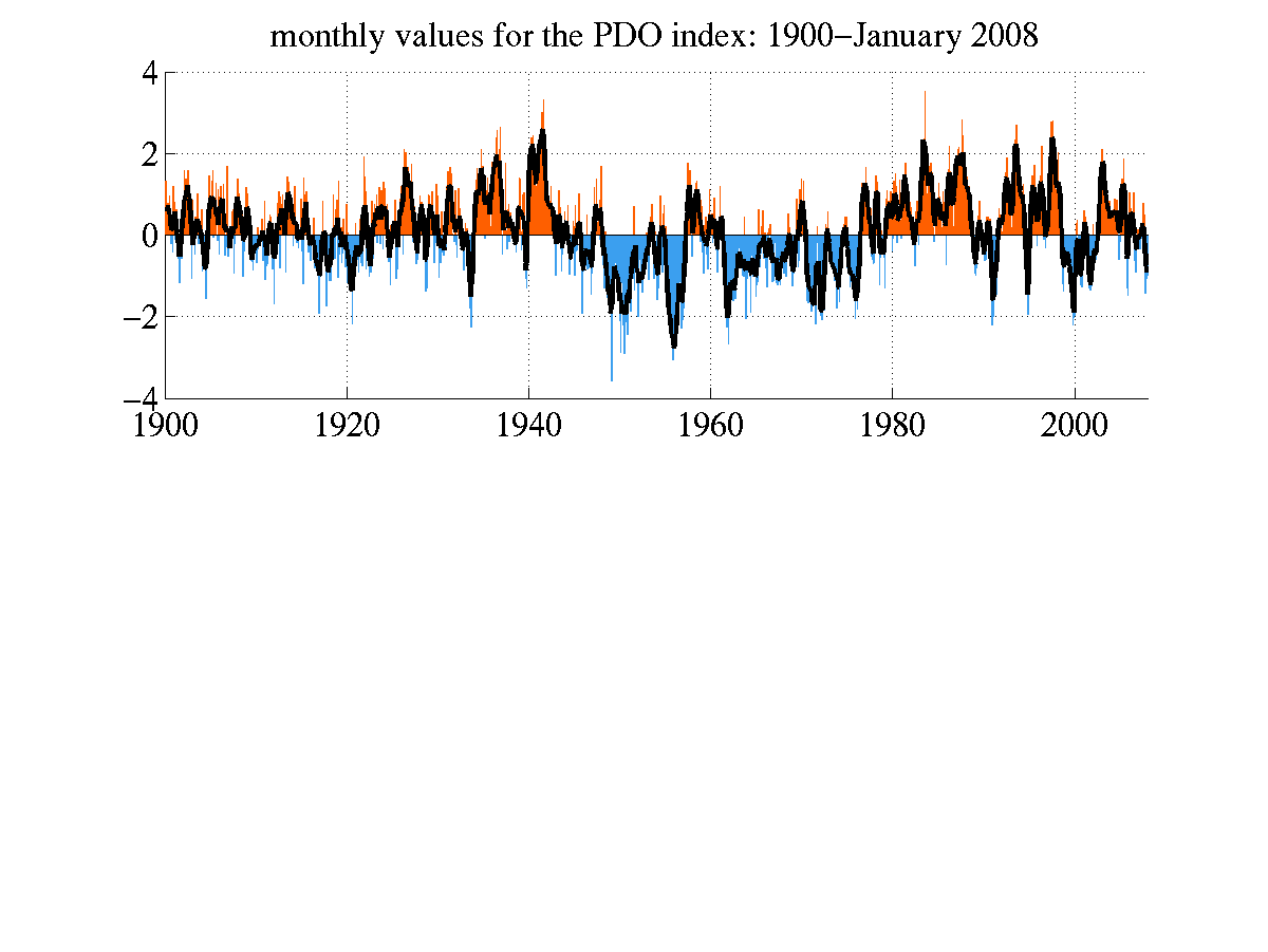
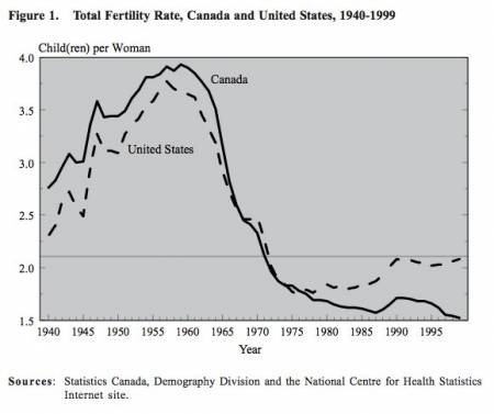
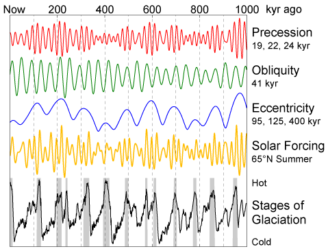
Below are some graphic examples of various time series data (some complicated, some simple) to illustrate the range of variations out there.

There are many, many ways to deal with time series data - many of them are complex, involving transforms of the data and the like. The mos common complex method invovles what is called a Fourier analsyis in which time series data can be transformed to produce fundamental frequncies:

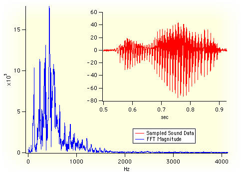
We will *not* be doing this because most environmental time series is too noisy to lend itself to this kind of analysis. Instead, we will guess what the frequencies will be.

To do this, we will be using simple sine waves (sinusoidal variations) to try and reproduce the time behavior of the data.

P(t) = A * sin((2π/ω)*t)

• A = amplitude
• ω = the inverse of the period (this is a frequency)

Note that the argument of sin is in units of radians not degrees.

So now we move to excel:

• On sheet 1 we have a template that will add together 3 different sine waves of arbitrary amplitude and period and then we automatically plot the sum of those 3 sine waves.

• On Sheet1 (2) we have the results of the three orbital cycle resonances. (Milankovitch cycles).

• On Sheet 2 we have some real El Nino Data to fit.

• On Sheet 3 we have idealized data (based loosely on eugene rain fall patterns). In this case we see sinusodial behavior superposed on a decreasing baseline. Thus we have to fit a linear + sine wave to get the right model.

  The reason for doing these kinds of fits is to extrapolate to the future which is why the model extends beyond the data so that predictions can be made.