There is simply no such thing as a perfect measurement or a perfect detector. All detectors/measurements have random noise associated with them.
The effect of random noise is that no two measurements are ever exactly
the same. Now, if the noise is sufficiently small, the average person
will not notice this effect in his or her every day life. Without such notice,
the individual labors under the illusion that measurements/science are
perfect To begin with, we will apply the concepts of errors to something that you care about – your exam scores!
On any exam, your score reflects two things:
These errors works like the following:
 What we measure is X, but what we are interested in is the distribution of the true variable, T. To measure T, however, we have to know what the random error, er and systematic error es is. Without knowledge of er and es, T can never be accurately measured. This potentially is a huge problem. What is er
 Random errors increase the variability around the mean. (In fact, this process in nature is what drives genetic evolution.) Random errors are associated with apparatus or method used in obtaining the data. All data sampling is subject to random error, period. There is no way to avoid it. You will definitely be dealing with random error and noise in this class. Note that in most detectors, random error is a fixed quantity so that the accuracy of the measurement depends upon the amplitude of the measured phenomena. For now, here is a simple example. Suppose I have a thermometer with a fixed random error of +/- 2 degrees. That is the accuracy of this device. Well, if its really 100 degrees out side, then this device will measure the temperature to an accuracy of 2% (2 out of 100). However, if its 20 degrees outside, the device will only measure the temperature to an accuracy of 10% (2 out of 20). What is es? (Systematic Error; often called calibration error).
 Systematic errors mean that different methods of measurement are being applied to the same variable. This means that the position of the mean is strongly effect. For example, suppose there are two patrolment on the freeway both with identical radar guns. Except that one of them systematically reads 5 mph higher than the other due to a "calibration" error back at the station. Which policeman do you want to speed by? Because of the presence of random error, it is always important to compare distributions via the method we have previously discussed (e.g. the Z-statistic)
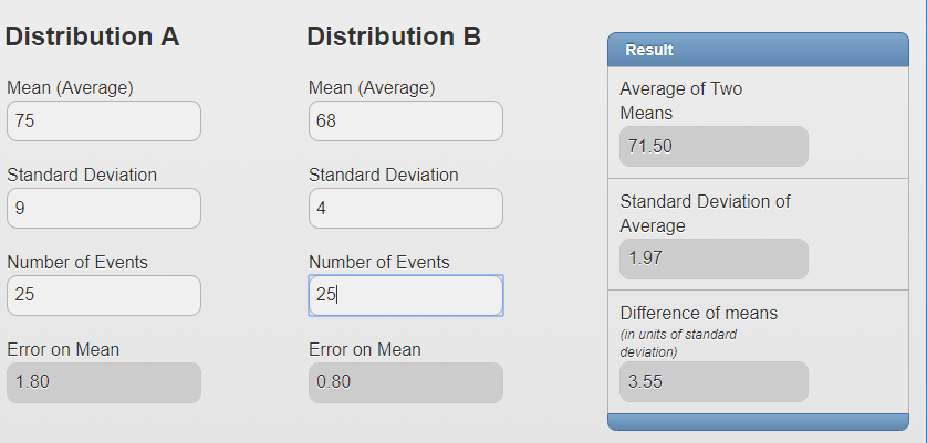
For example comparing two identically structured midterms with 25 students in a class.
 The Z-test says the difference between these two exams is marginally significant. Therefore, the exams should not weight equally in the determination of the grade. The likely difference between the two midtermas is that grading techniques have been better learned so the amount of random grading error is less on the second midterm. Now if the class size were 100 students, the difference between these two exams would be quite significant. 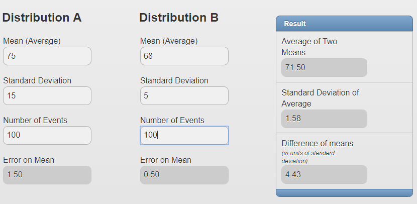 This shows that often times a relatively large N is needed to overcome the random or intrinsic noise in a system for differences to be properly measured. Now, suppose that, for the first midterm, we know that the random error was 12 points and for the second midterm, the random error is 3 points. We will show below that, compensating for this random error, will now produce a significant difference between these two exam distributions.
 Here is how you subtract out a known random error. In a bell-shaped distribution, the various components are added or subtracted in quadrature. What does that mean?:
so (true σ )2 = (measured σ )2 - er2 Now we apply this to the case of our two exams:
Now what is the z-statistic?
 Now a significant difference emerges from the example when the random (grading) error is accounted for. In the raw data, this significance is obscured by the large amount of random error. This is a real life problem which is why its important to try and assess how much random error exists in your sample or data before you reach any conclusions about one distribution being different than the other. .
Understanding the role of measurement errors is crucial to proper data interpretation. For instance, the measured dispersion in some distribution represents the convolution of
In general, you don't want to have the observed value of σ dominanted by measurement error or poor instrumental precision because then you can't draw any valid conclusion. This is particularly a problem in working with climate change data. Example: Column 1 contains the data that was measured with good precision. That is, the measuring error of the instrument was less than 0.1. Column 2 represents the same data that was measured with and instrument that had a measuring error of +/- 1 unit:
The first column yields σ = 0.23. The second column yields σ = 1.44. Clearly, the first column is a better measure of the intrinsic distribution of the sample than the second column. Essentially the numbers in the second column are meaningless – because they are dominated by random error due to the imprecise way the quantity was measured. Note, that your GPA is actually determined in a rather imprecise way. Your GPA is recorded to an accuracy of 2 digits (e.g. 3.14). Yet each class is measured far more coarsely (to within a precision of 0.3 grade points). The second decimal place in your GPA is essentially meaningless, because the instrument that grades you is not sufficiently precise to render meaning to a two decimal place GPA. Yet it perpetuates and serves as another good example for the failure of science to inform policy. Every measurement has an error associated with it and hence a measurement is only as good as its error. Knowing the size of measuring or sampling errors is often difficult, but it still is important to try and determine these errors. For some kind of sampling, error estimation is straightforward. For instance, opinion poll sampling has an error that depends only on the number of people in the sample. This error has to do with counting statistics and is expressed as
For a sample of 16 people, the error would be 4/16 = 25%. This a large error since the range of YES vs. NO is from 0-100% if 12 people answered yes and 4 people answered no then your result would be:
For a sample of 1000 people, the error would be SQRT(1000)/1000 = 33/1000 = 3%. If 750 answered yes and 250 answered no then your result would be:
which now shows that Yes is significant over No
|
 Nothing could be further from the truth.