The Z-test
To compare two different distributions one makes use of a tenant of statistical theory which states that
The error in the mean is calculated by dividing the dispersion by the square root of the number of data points.
In the above diagram, there is some population mean that is the true intrinsic mean value for that population. We can never measure that population directly. Instead, we sample (and we better be randomly sampling) that population by reaching into it (in the above image we have formed 8 separate samples) and getting various samples, each of which are defined by some sample mean:

If we have truly randomly sampled the parent population, then there should be no significant differences among the 8 sample means that we have obtained. This is one way you can use to determine, in fact, the likelihood that your sample means it a good indicator of the true population mean.
The error in the mean can be thought of as a measure of how realiable a mean value has been determined. The more samples you have, the more reliable the mean is. But, it goes as the square root of the number of samples! So if you want to improve the reliability of the mean value by, say, a factor of 10, you would have to get 100 times more samples. This can be difficult and often your stuck with what you got. You then have to make use of it.
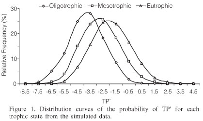
Ultimately, the purpose of this test is to see if two distributions are significantly different from one another. For instance, the three distributions below do overlap with one another, somewhat – does that mean they are the same or are they different? Remember, statistically significant differences mean that whatever the conditions are that determine one distribution, they are not the same as the conditions that produce the other distribution. (These points will become more clear to you in the second homework assignment when you work through some actual examples.)
The Z-test is especially useful in the case of time series data where you might want to assess a "before and after" comparison of some system to see if there has been effect. One relevant example (which you will do on the second assignment) is to determine whether or not "grade inflation" is real and statistically significant.
It is often said that you can only use the Z-test when you have a sample that you're comparing against a parent population of known mean and standard deviation. This is not really true – you can always use the z-test when comparing two samples.
Comparing Two Sample Means – Find the difference of the two sample means in units of sample mean errors. Difference in terms of significance is:
But for comparing two samples directly, one needs to compute the Z statistic in the following manner:
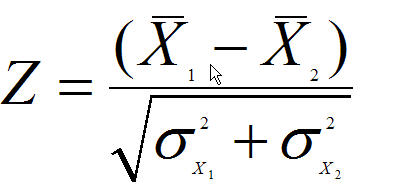
Where
Here is a specific example of the Z-test application:
Eugene vs. Seattle rainfall comparison over 25 years (so N = number of samples = 25):
| Eugene | Seattle |
|---|---|
| mean = 51.5 inches | mean = 39.5 inches |
| dispersion = 8.0 | dispersion = 7.0 |
| N = 25 | N = 25 |
| error in mean = 8.0/5 | error in mean = 7.0/5 |
| error in mean = 1.6 | error in mean = 1.4 |
So far this example:
Therefore, the Z-statistic is 12/2.1 = 6  which means there is
a highly significant difference between these two distributions which means it
really does rain significantly more in Eugene than in Seattle.
which means there is
a highly significant difference between these two distributions which means it
really does rain significantly more in Eugene than in Seattle.
You can verify these numbers by using the Z-test tool (comparing two means) accessible from the statistical tools area.
In general, in more qualitative terms:
In many fields of social science, the cricital value of Z (Zcrit) is 2.33 which represents p =0.01 (shaded area below has 1% of the total area of the probability distribution function). This means the two distributions have only a 1% probability of being actual the same.