

Example:
If the events occur on average every 4 minutes, and you are interested in the number of events occurring in a 10 minute interval, you woulduse a Poisson distribution with λ = 2.5.
(e.g. 10/4
 total time window divided by average arrival rate). So say in one sample you detected 6 events in that 10 minute window, so x=6. Plug those numbers directly in to the calculator.
The calculator returns a probablity of 2.7% that there would be 6 events in this 10 minute window indicating that to be an unlikely occurrence (note you can ignore the other returned probablities).
In a Poisson distribution:
This distribution arises as a consequence of the summation of many rare events.
Examples of environmentally related events governed by this distribution:
 Poisson statistics govern the behavior of queues!
Some important assumptions
Lollipops arrive to the lollipop tester on average every 10 minutes.
The arrival process is Poissonian.
What is the probability of 2 arrivals in the next 15 minutes?
So, x =2 (that's the number of events we are counting)
λ = 1.5 (we expect one per arrival every 10 minutes; total time = 15 minutes;
&lambda = 15/10 = 1.5)
P(x) = .251
What about 4 events?
P(x) = .047
Another Example:
Assume that the probability of dying from leukemia is described by a Poisson
distribution with a mean of 2.3 deaths per 10000 children
You now have been commissioned to study an apparent increase in leukemia
incidences associated with children that live in ToxicWasteVille. Your boss,
The Federal Health Authority, has determined that compensation will be based on
a 1% criteria - that is, if the probability of the increase in occurrence is
less than 1% then they will be compensated.
Your qualitative bias is to be on the side of the children.
You then go to ToxicWasteVille and measure a local death rate of 6 deaths per
10000 children. That is you observed 6 events (X = 6) when the
expected event rate was 2.3. Important, you can not observe
fractional events!
Will this death rate qualify for compensation?
P(6) = e-2.3 2.36 / 6! P(6) = 0.1003 * 148.04 / 720 P(6) = 0.021 or 2.1% Note: the Poisson distribution would not be used with an infectious disease
because the events (people with the disease) would not be independent of each
other, i.e. if your partner has an infectious disease the probability of you
getting it is higher than some one not in contact with the disease.
Example:
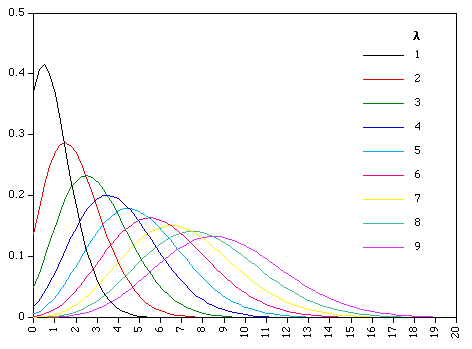
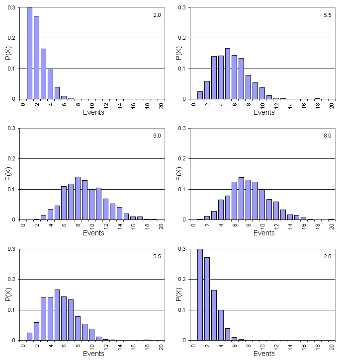
The following animation shows the probability distribution of events
as a function of λ (shown in upper right hand corner)  you can see as λ increases the probability distribution
evolves from being skewed to being normal. this means for large x (x>20 or so) you can just use normal distributions and standard deviations to determine probabilty of occurence).

Determining the probability of a rare event
So,
What is the probability
of observing a local death rate of 6 deaths per 10000?
 λ = 2.3
 does not meet
the compensation criteria
Last example (I have used in a climate change paper) was the 2005 Hurricane season in which there were 3 Cat 5 Hurricanes (Katrina, Rita and Wilma) the occured within a 6 week period in the Gulf of Mexico: