Exercise 4: Visiting Santa Claus in a Canoe



This assignment will center common elements of working with time series data: smoothing of noisy data, feature extraction, curve fitting, and long term prediction from TIME SERIES data.




Instructions:

1. Get the Data File This data is a measure of summer season Arctic Sea Ice Extent.
   • Column 1 = year
   • Column 2 = July
   • Column 3= August
   • Column 4 = September
   
   
   All listed units are in in square kilometers.
   
   While again you may use any application that you like, some of the requirments below can not easily be meet with shoving the data into Matlab or Mathematica. There will be some custom coding needed to complete all of the required aspects.
   
   
2. Average the 3 months for each year and then plot that time series. Differentiate (dy/dt) this curve in 5 years intervals and plot the resulting slope vectors vs time.
   
   
3. Smooth the average data from above:
   
   
   • box car (moving average) of width 5 years
   • Gaussian kernel of width 7 years
   • Exponential smoothing
   
   
   Plot all three smoothing waveforms on the same graph and comment on any differences that you notice in smoothing procedure.
   
   
4. Plot a histogram of the yearly ratios between July and September Sea Ice Extent and comment on any pattern that you might notice.
   
   
5. There are a few scientists who believe that the recent behavior in the Arctic is consistent with previous cycles of warming and cooling. Prior to 1975 there are two suggested cooling periods which allow the Summer Sea Ice Extent to remain larger than average. To extract these features from the data, requires data windowing and baseline subtraction. This is a common form of "spectral feature analysis".
   
   This means fitting a baseline (a polynomial fit is fine here as in this case the baseline represents some sort of instrumental noise) outside the window and then subtracting out that baseline to flatten the spectra. An example from radio astronomy is shown here.
   
   

   the (emission) feature (positive) is windowed and a baseline is fit to the data outside the window and subtracted to produce a flat baseline plus feature. The area under the feature is of interest.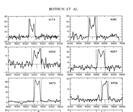

   
   
   There are supposedly two events in this data set of this cooling producing heigher than average sea ice extents for a few years. By this method just outlined, determine the total area of each event (you will have to decide when the event begins and ends).
   
   
6. When do we melt Santa's Home
   
   Use only the satellite data, which starts in 1979 and use only the September data. You will probably want to smooth that raw data. Now, using any technique that you want, except fitting this curve with a polynomial since nothing in nature is a polynomial, predict in what year the September ice extent will reach 0 square kilometers. Produce a plot of your fit to the data.