Upload the assignment here

Exercise 4: Visiting Santa Claus in a Canoe



This assignment will center on another common element of working with data, namely feature extraction, curve fitting, and long term prediction from TIME SERIES data. This exercise involves less than the previous ones and correspondingly there is an expectation for the whole thing to be finished by thursday at 10 pm. You are ENCOURAGED to do this project collaboratively by sharing code on GITHUB. For instance, your team might divide itself among the SEVEN tasks below. Bootstrap would be an excellent way to present your overall results.

Instructions:

1. Get the Data File This data is a measure of summer season Arctic Sea Ice Extent.
   • Column 1 = year
   • Column 2 = July
   • Column 3= August
   • Column 4 = September
   
   
   All listed units are in in square kilometers.
   
   While again you may use any application that you like, some of the requirments below can not easily be meet with shoving the data into Matlab or Mathematica. There will be some custom coding needed to complete all of the required aspects.
   
   
2. Average the 3 months and then differentiate (dy/dt) this curve in 5 years intervals and plot the resulting slope vectors - this can be done using a finite difference approach or any number of ways.
   
   
3. Using any numerical integration technique that you like, compute the total area of the curve from 1870 to 1950 and compare that to the area under the curve from 1950 to 2013.
   
   
4. Using the information contained HERE smooth the wave form via
   • box car (moving average) of width 5 years
   • Gaussian kernel of width 5 years
   • Exponential smoothing with greatest weight given to the last 20 years
   
   
   Plot all three waveforms on the same graph and comment on any differences that you notice in smoothing procedure.
   
   
5. Plot a histogram of the yearly ratios between July and September Sea Ice Extent and comment on any pattern that you might notice.
   
   
6. There are a few scientists who believe that the recent behavior in the Arctic is consistent with previous cycles of warming and cooling. Prior to 1950 there are two suggested cooling periods which allow the Summer Sea Ice Extent to remain larger than average. To extract these features from the data, requires data windowing and baseline subtraction. This is a common form of "spectral feature analysis".
   
   This means fitting a baseline (a polynomial fit is fine here as in this case the baseline represents some sort of instrumental noise) outside the window and then subtracting out that baseline to flatten the spectra. An example from radio astronomy is shown here.
   
   

   the (emission) feature (positive) is windowed and a baseline is fit to the data outside the window and subtracted to produce a flat baseline plus feature. The area under the feature is of interest.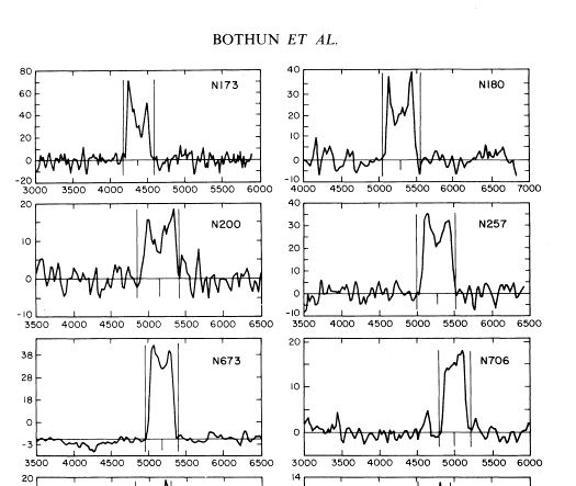

   
   
   There are supposedly two events in this data set of this cooling producing heigher than average sea ice extents for a few years. By this method just outlined, determine the total area of each event (you will have to decide when the event begins and ends) and compare that to the average area from the period 1870 to 1950, that you determined previously, to determine the overall amplitude of this cooling.
   
   
7. When do we melt Santa's Home
   
   You are to make this determination using two sets of data.
   
   
   • a) Using the entire data set, determine a smooth functional form that best fits the data an extrapolate that to zero to determine when Norwegian Cruise lines should be taking bookings. DO NOT USE A POLYNOMIAL fit in this case. Nothing in nature is fit by a POLYNOMIAL. Produce a graph with your fitted line to the data, exptrapolated to zero.
     
     
   • b) Now use only the satellite data, which starts in 1979 and use only the September data. Fit a linear regression to the data (you can use any package you want for that) but then also fit some kind of power or exponential law to the data. You will find the two zero predictions to be quite different and once of them is scary. Plot those two fits on the same graph.
     
     Although this is an extreme case, the following is an example of the kind of power law or damped exponential fit that the data may lend itself to
     
     
     
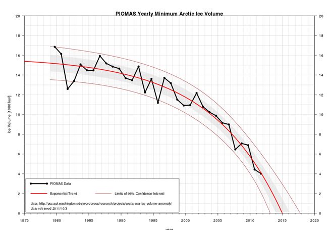
     Real life Note: This is currently a strongly debated situation in the climate science world. The linear argument is that, yes there is a problem, but its not that severe. The power law fit would argue that we have reached a tipping point and we better start thinking. Note, the military already has an extensive plan for a Navigable Artic Ocean .
     
     Read This account and pay particular attention to the paragraph about EXCELLENCE.
     
     
     • This is due by 10 pm on Thursday May 1

In class on May 2 we will discuss this assignment and extract a little science as well.