HW 4a

In Part I we will be concerned with the basics of least squares fitting and weighted fitting as applied to real data. Much of this might seem overly simplistic to you but it will come in handy at some future point in your career.

Also note that in this assignment, the very last step will be the most time intensive.

Steps:

Download the two column data set Yes the units are kind of ridiculous in this data; this doesn't matter.

Write your own least squares fitting program. This doesn't mean writing something that sources class libraries; code the math yourself! Now feed the data set to your elegant code and include the fitted equation, scatter around the relation, and the plot showing the fitted line to the data as well as your code

you should find:

slope ~ 11900
intercept ~ 2810;
σ ~900;

If you compare your output with any other standard regression program, there will be slight numerical differences for this data set since it determines a numerically high value for the slope.

Add to your code the necessary lines to now compute the error in the slope. From the two error lines now report the predicted value for X=1.2 and its uncertainty

Now add to your code the necessary lines to compute the χ². Report the χ² value

Produce and submit a residual plot

Now go through one cycle of 2.5σ clipping and redo the above steps to report on the improved precision that you know have for the X=1.2 predicted value as well as the χ² value

Now we will work on weighted averages using the noise associated with the data.

Download the global temperature data . From this data set, compute the average and standard deviation (no you don't have to write your own program for this) of the Y-variable (which is a temperature anomoly) in 9 year time intervals starting with 1880. Note that this averaging will not include the 2015 and 2016 data values - we will use thos separately later. Your X value should be the time midpoint of the averages, e.g. 1884.5, 1913.5, etc.

Run your least squares program and produce the best fitting line (and this relation is not linear, do not worry about that) Submit the relevant plot and report on the slope of the line

Now add code that allows you to determine a weighted least squares fit where the weights go as the inverse square of the noise associated with your decadel averages). Submit the relevant plot and comment on whether or not the weighting has made a difference. In particular did the elops of the line change significantly?

Now return to the unweighted fitted averages and add the last two data points in (2015 and 2016). Did the slope of the line change significantly? How many σ off the regresion line are these last two points? Predict the value for the year 2050.

Now you, the data scientist, wants to sell policy. You assume that most of the power in this relation is in the last few data points. So weight the data by Y² and now predict the value for the year 2050. Has the slope of the line now changed significantly from the original fit to the unweighted data

Now we want to fit a non-linear curve to this data. We are going to choose what is often called a 4PL function or a symmetric sigmoidal. The form of this function is

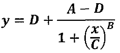
This function has 4 variables: a,b,c,d Using the method of χ² minimization, find the best values for a,b,c,d. Yes you can find a curve fitter somewhere to probably do the work for you but I want you to use the method of guess and check to find the values which minimize χ².

To help you converge fast, since these values can be really strange numerically. I will give you ranges for the a,b,c,and d parameters.

a: between -0.4 and -0.2
b: between 40 and 80
c: between 2000 and 3000
d: between 300000 and 400000 (d is always a weird number)

Produce the best fitting 4PL plot and now 1) predict the value in the year 2050 2) compare your value of chi;² for this model compared to the linear model