Start off by please trying to do the last part of the previous homework.

Now we want to fit a non-linear curve to this data. We are going to choose what is often called a 4PL function or a symmetric sigmoidal. The form of this function is



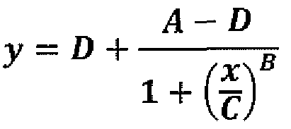
This function has 4 variables: a,b,c,d Using the method of χ² minimization, find the best values for a,b,c,d. Yes you can find a curve fitter somewhere to probably do the work for you but I want you to use the method of guess and check to find the values which minimize χ².

To help you converge fast, since these values can be really strange numerically. I will give you ranges for the a,b,c,and d parameters.

• a: between -0.4 and -0.2
• b: between 40 and 80
• c: between 2000 and 3000
• d: between 300000 and 400000 (d is always a weird number)

Produce the best fitting 4PL plot and now 1) predict the value in the year 2050 2) compare your value of chi;² for this model compared to the linear model



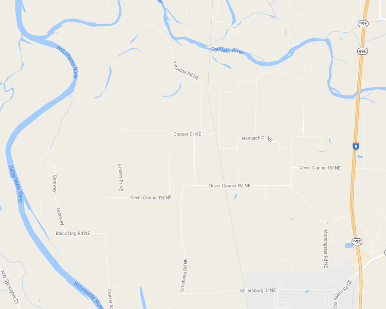
In part II we are going to use river guage levels for the main tributaries of the Willamette River over the period Jan 1 - April 30. We will do several things in terms of trend extrapolation with this data. Note of course, in real life, your predicted floods and/or flows are now highly controlled through the Dam and Levy system. However, in the real world the floodplains of the Willamette are quite extensive. If you want to ride your bike around the best vestiage of these flood plains see this region North of Albany and South of the Santiam River .

Indeed the Willamette river floods of, 1861, 1894, and 1964 are pretty significant. For some of the science behind floor prediction etc, consult this reference

Steps:

1. Get the data file This data set is about 200,000 lines long and has 5 fields:
   
   
   • River Name and Geographic Location
   • Latitude and Longtitude of Flood Gauge
   • Timestamp
   • Gauge Level (in Feet)
   
   
   Using Google Earth or something else, produce a map of flood gauge locations relative to the Willamette River
   
   
2. Some List Management:
   
   In the raw file data is recorded every 15 minutes. We don't need that high of time resolution for most of this exercise (we will only use it in the case of an "event"). You will therefore want to bin all the time data into 3 hour values (8 measurements per day). You will also want to convert to a timestamp in units of hours from January 1, 2017 (ignore or delete any data in the file that precedes this date). Finally, you will prepare separate data files for each unique river name (this unqineness is defined by the names that come before the word "river" - hence North Santiam, South Santiam, and Santiam, are 3 independent rivers). Include a directory listing of your filenames and the number of lines in each file
   
   For this part, you will aggegrate all the individual gauges for each river:
   
   
3. Determine the river which has the lowest and highest MEDIAN values for levels over the time period Jan 1 - Apr 30. Produce a plot of both those rivers and determine the maximum slope that exists in each case
   
   
4. For each river, define an "alarm event" in which the river stage is two times higher than the minimum gauge level in this time period. For each river, produce the duration times when these high levels are maintained. Comment on any differences you see between the rivers
   
   
5. For each river, find the maximum peak in the data and plot the time step of the peak against latitude (where latitude is the average of all the individual gauge latitudes on that river).
   
   For this part, we will now be concerned with individual gauges on each of the rivers.
   
   
6. For each river determine which gauge is closest to the Willamette River and which is farthest. a) Determine the distance between these gauges and Produce a histogram of those distances and b) determine the average level difference between these two gauges at minimum gauge stage for each and Produce a histogram of those level differences
   
   
7. Now lets focus on the March 8 "event".
   
   
   • a) Determine the slope of the gauge river rise from 00 hours on March 8 until the time of the peak for the UPPER guage. Predict what the peak amount will be on the LOWER guage and compare that to the actual observation. Produce a histogram of the differences between prediction and observation
     
     
   • b) Now for this March 8 event, go back to original data file and use the 15 minute time interval data, again up until the time of maximum peak. From that data produce plots for the LOWER guage that include both linear and non-linear fits and their respective χ² values
     
     
   • Finally we now want to estimate the total impact on Downtown Portland under the following assumptions:
     
     
     • 60% of the total river level in downtown portland is determined by the combined heights of these rivers at the LOWER flood guage.
       
       
     • The March 8 event will persist for 5 more days, from the locally high peak that you measured at the UPPER river guage (this actully will simulate the 1996 Willametter River Valley Floods)
     
     
     
   • c) Predict how much higher the river level will be after these extra 5 days and determine if the water level is now over the river wall in downtown portland (and it was over the wall in the 1964 flood before Lookout Point reservoir was built).