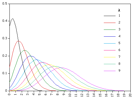
The probability that there are x occurences of an event (where x is a non-negative integer is given by)

λ is often a rate per unit time, distance, or area. This is a discrete distribution based on counting events. Note as you tend towards large λ (i.e. long times) this distribution becomes like a normal distribution.

This distribution arises as a consequence of the summation of many rare events. Examples of events governed by this distribution:

• The number of cars that pass through a certain point on a road during a given period of time.

• The number of spelling mistakes a secretary makes while typing a single page.

• The number of phone calls at a call center per minute Poisson statistics govern the behavior of queues!

• The number of roadkill found per unit length of road

• The number of pine trees per unit area of mixed forest.

• The number of soldiers killed by horse-kicks each year in each corps in the Prussian cavalry.

• The number of Cat 5 Hurricanes that pass by a given latitude and longtitude

Some important assumptions

• arrivals/events occur one at a time (hence discrete)

• probability of an arrival/event in a given time interval depends only on the length of the time interval

• the number of arrivals/events in non-overlapping times intervals are independent - that is the arrival of the next event is not correlated with the fact that a previous event has occurred. This is important. If this is not the case, then you can not use this statistical approach.

Example:

Lollipops arrive to the lollipop tester on average every 10 minutes.

The arrival process is Poissonian.

What is the probability of 2 arrivals in the next 15 minutes?

So, x =2 (that's the number of events we are counting)

λ = 1.5 (we expect one per arrival every 10 minutes; total time = 15 minutes; λ = 15/10 = 1.5)

P(x) = .251

What about 4 events?

P(x) = .047