Summary:
A collection of data (hopefully randomly sampled) is usually called a sample or
a population (of data). From that sample/population one can construct the basic
sample/population statistics:
The Sample/Population Mean –
Numerical measure of the average or most probable value in some distributions.
Can be measured for any distribution. Knowing the mean value alone for some
sample is not very meaningful.
The Sample/Population Distribution – Plot of the frequency of occurrence of ranges of data values in the sample. The
distribution needs to be represented by a reasonable number of data intervals
(counting in bins).
The
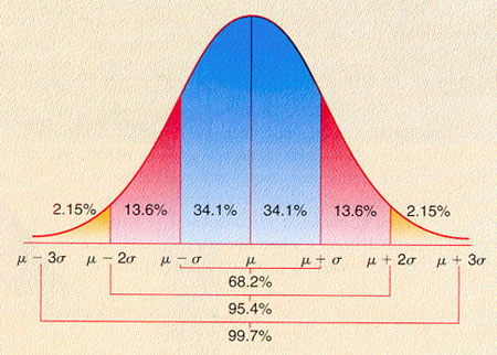
Sample Dispersion or standard deviation – Numerical measure of the range of the data about the
mean value. Defined such that +/- 1 dispersion
unit contains 68% of the sample, +/- 2 dispersion units contains 95% and +/- 3
dispersion units contains 99.7%. This is schematically shown below:

In general, we map dispersion/standard deviation units on to
probabilities: http://zebu.uoregon.edu/2003/es202/ptable.html.
For instance:

- The probability that some event will be greater
than 0 dispersion units above the mean is 50%.
- The probability that some event will be greater
than 1 dispersion unit above the mean is 15%.
-
The probability that some event will be greater
than 2 dispersion units above the mean is 2%.
- The probability that some event will be greater
than 3 dispersion units above the mean is 0.1% (1 in 1000).
The above is an approximation but its fine. The more exact
values are shown below:
For our purposes, risk assessment of natural hazards, we only care about order of magnitude probabilities; i.e. 1 in 10, 1 in 100, 1 in 1000, etc.
The
calculation of dispersion (standard deviation) in a distribution is very important because it
represents a uniform way to determine probabilities and therefore to determine
if some event in the data is expected (i.e., probable) or is significantly
different than expected (i.e., improbable).
Sampling
|